MRECW Students E- Learning Point Computer Security Student (CSS)

Tuesday 6 October 2015

Sorting

7 Sorting
Sorting is one of the most important operations performed by computers. In the days of magnetic tape storage before modern data-bases, it was almost certainly the most common operation performed by computers as most "database" updating was done by sorting transactions and merging them with a master file. It's still important for presentation of data extracted from databases: most people prefer to get reports sorted into some relevant order before wading through pages of data!

7.1 Bubble, Selection, Insertion Sorts

There are a large number of variations of one basic strategy for sorting. It's the same strategy that you use for sorting your bridge hand. You pick up a card, start at the beginning of your hand and find the place to insert the new card, insert it and move all the others up one place.

/* Insertion sort for integers */

void insertion( int a[], int n ) {
/* Pre-condition: a contains n items to be sorted */
    int i, j, v;
    /* Initially, the first item is considered 'sorted' */
    /* i divides a into a sorted region, x<i, and an
       unsorted one, x >= i */
    for(i=1;i<n;i++) {
        /* Select the item at the beginning of the
           as yet unsorted section */
        v = a[i];
        /* Work backwards through the array, finding where v 
           should go */
        j = i;
        /* If this element is greater than v,
              move it up one */
        while ( a[j-1] > v ) {
          a[j] = a[j-1]; j = j-1;
          if ( j <= 0 ) break;
          }
        /* Stopped when a[j-1] <= v, so put v at position j */
        a[j] = v;
        }
    }

Bubble Sort

Another variant of this procedure, called bubble sort, is commonly taught:

/* Bubble sort for integers */
#define SWAP(a,b)   { int t; t=a; a=b; b=t; }

void bubble( int a[], int n )
/* Pre-condition: a contains n items to be sorted */
    {
    int i, j;
    /* Make n passes through the array */
    for(i=0;i<n;i++)
        {
        /* From the first element to the end
           of the unsorted section */
        for(j=1;j<(n-i);j++)
           {
           /* If adjacent items are out of order, swap them */
           if( a[j-1]>a[j] ) SWAP(a[j-1],a[j]);
           }
        }
    }

Analysis

Each of these algorithms requires n-1 passes: each pass places one item in its correct place. (The n^th is then in the correct place also.) The i^th pass makes either ior n - i comparisons and moves. So:

or O(n²) - but we already know we can use heaps to get an O(n logn) algorithm. Thus these algorithms are only suitable for small problems where their simple code makes them faster than the more complex code of the O(n logn) algorithm. As a rule of thumb, expect to find an O(n logn) algorithm faster for n>10 - but the exact value depends very much on individual machines!. They can be used to squeeze a little bit more performance out of fast sort algorithms -

Key terms

Bubble, Insertion, Selection Sorts: Simple sorting algorithms with O(n²) complexity - suitable for sorting small numbers of items only.

Binary Sort

7.4 Bin Sort
Assume that in the bin sort

the keys of the items that we wish to sort lie in a small fixed range and
that there is only one item with each value of the key.

Then we can sort with the following procedure:

Set up an array of "bins" - one for each value of the key - in order,
Examine each item and use the value of the key to place it in the appropriate bin.

Now our collection is sorted and it only took n operations, so this is an O(n) operation. However, note that it will only work under very restricted conditions.

Constraints on bin sort

To understand these restrictions, let's be a little more precise about the specification of the problem and assume that there are m values of the key. To recover our sorted collection, we need to examine each bin. This adds a third step to the algorithm above,

Examine each bin to see whether there's an item in it.

which requires m operations. So the algorithm's time becomes: T(n) = c₁n + c₂m and it is strictly O(n + m). Now if m <= n, this is clearly O(n). However if m >> n, then it is O(m). For example, if we wish to sort 10⁴ 32-bit integers, then m = 2³² and we need 2³² operations (and a rather large memory!).
For n = 10⁴:

nlogn ~ 10⁴ x 13 ~ 2¹³ x 2⁴ ~ 2¹⁷ So quicksort or heapsort would clearly be preferred. An implementation of bin sort might look like:

#define EMPTY -1 /* Some convenient flag */
void bin_sort( int *a, int *bin, int n ) {
    int i;
    /* Pre-condition: for 0<=i<n : 0 <= a[i] < M */
    /* Mark all the bins empty */
    for(i=0;i<M;i++) bin[i] = EMPTY;
    for(i=0;i<n;i++)
        bin[ a[i] ] = a[i];
    }

main() {
    int a[N], bin[M];    /* for all i: 0 <= a[i] < M */
    .... /* Place data in a */
    bin_sort( a, bin, N );

If there are duplicates, then each bin can be replaced by a linked list. The third step then becomes:

Link all the lists into one list.

We can add an item to a linked list in O(1) time. There are n items requiring O(n) time. Linking a list to another list simply involves making the tail of one list point to the other, so it is O(1). Linking m such lists obviously takes O(m) time, so the algorithm is still O(n+m). In contrast to the other sorts, which sort in place and don't require additional memory, bin sort requires additional memory for the bins and is a good example of trading space for performance.

Although memory tends to be cheap in modern processors -
so that we would normally use memory rather profligately to obtain performance,
memory consumes power
and in some circumstances, eg computers in space craft,
power might be a higher constraint than performance.

Having highlighted this constraint, there is a version of bin sort which can sort in place:

#define EMPTY -1 /* Some convenient flag */
void bin_sort( int *a, int n ) {
    int i;
    /* Pre-condition: for 0<=i<n : 0 <= a[i] < n */
    for(i=0;i<n;i++)
 if ( a[i] != i )
            SWAP( a[i], a[a[i]] );
    }

However, this assumes that there are n distinct keys in the range 0 .. n-1. In addition to this restriction, the SWAP operation is relatively expensive, so that this version trades space for time. The bin sorting strategy may appear rather limited, but it can be generalised into a strategy known as Radix sorting.

Radix

7 Radix Sorting
The bin sorting approach can be generalised in a technique that is known as radix sorting.

An example

Assume that we have n integers in the range (0,n²) to be sorted. (For a bin sort, m = n², and we would have an O(n+m) = O(n²) algorithm.) Sort them in two phases:

Using n bins, place a_i into bin a_i mod n,
Repeat the process using n bins, placing a_i into bin floor(a_i/n), being careful to append to the end of each bin.

This results in a sorted list. As an example, consider the list of integers:

36 9 0 25 1 49 64 16 81 4

Bin	0	1	2	3	4	5	6	7	8	9
Content	`0`	`1 81`	-	-	`64 4`	`25`	`36 16`	-	-	`9 49`

n is 10 and the numbers all lie in (0,99). After the first phase, we will have: Bin 0 1 2 3 4 5 6 7 8 9 Content 0 1 81 - - 64 4 25 36 16 - - 9 49 Note that in this phase, we placed each item in a bin indexed by the least significant decimal digit.
Repeating the process, will produce:

Bin	0	1	2	3	4	5	6	7	8	9
Content	`0 1 4 9`	`16`	`25`	`36`	`49`	`-`	`64`	`-`	`81`	`-`

In this second phase, we used the leading decimal digit to allocate items to bins, being careful to add each item to the end of the bin.
We can apply this process to numbers of any size expressed to any suitable base or radix.

7.5.1 Generalised Radix Sorting

We can further observe that it's not necessary to use the same radix in each phase, suppose that the sorting key is a sequence of fields, each with bounded ranges, eg the key is a date using the structure:

typedef struct t_date {
    int day;
    int month;
    int year; 
} date;

If the ranges for day and month are limited in the obvious way, and the range for year is suitably constrained, eg 1900 < year <= 2000, then we can apply the same procedure except that we'll employ a different number of bins in each phase. In all cases, we'll sort first using the least significant "digit" (where "digit" here means a field with a limited range), then using the next significant "digit", placing each item after all the items already in the bin, and so on. Assume that the key of the item to be sorted has k fields, f_i|i=0..k-1, and that each f_i has s_i discrete values, then a generalised radix sort procedure can be written:

radixsort( A, n ) { for(i=0;i<k;i++) { for(j=0;j<s_i;j++) bin[j] = EMPTY;	O(s_i)
for(j=0;j<n;j++) { move A_i to the end of bin[A_i->f_i] }	O(n)
for(j=0;j<s_i;j++) concatenate bin[j] onto the end of A; } }	O(s_i)

Total

Now if, for example, the keys are integers in (0,b^k-1), for some constant k, then the keys can be viewed as k-digit base-b integers.
Thus, s_i = b for all i and the time complexity becomes O(n+kb) or O(n). This result depends on k being constant.
If k is allowed to increase with n, then we have a different picture. For example, it takes log₂n binary digits to represent an integer <n. If the key length were allowed to increase with n, so that k = logn, then we would have:

.
Another way of looking at this is to note that if the range of the key is restricted to (0,b^k-1), then we will be able to use the radixsort approach effectively if we allow duplicate keys when n>b^k. However, if we need to have unique keys, then k must increase to at least log_bn. Thus, as n increases, we need to have logn phases, each taking O(n) time, and the radix sort is the same as quick sort!

Sample code

This sample code sorts arrays of integers on various radices: the number of bits used for each radix can be set with the call to SetRadices. The Bins class is used in each phase to collect the items as they are sorted. ConsBins is called to set up a set of bins: each bin must be large enough to accommodate the whole array, so RadixSort can be very expensive in its memory usage!

Quickk Sort

Quick Sort

Features

Similar to mergesort - divide-and-conquer recursive algorithm
One of the fastest sorting algorithms
Average running time O(NlogN)
Worst-case running time O(N²)

Basic idea

Pick one element in the array, which will be the pivot.
Make one pass through the array, called a partition step, re-arranging the entries so that:

the pivot is in its proper place.
entries smaller than the pivot are to the left of the pivot.
entries larger than the pivot are to its right.

Recursively apply quicksort to the part of the array that is to the left of the pivot,
and to the right part of the array.

Algorithm

STEP 1. Choosing the pivot
Choosing the pivot is an essential step.
Depending on the pivot the algorithm may run very fast, or in quadric time.:

Some fixed element: e.g. the first, the last, the one in the middle

Randomly chosen (by random generator ) - still a bad choice.
The median of the array (if the array has N numbers, the median is the [N/2] largest number. This is difficult to compute - increases the complexity.
The median-of-three choice: take the first, the last and the middle element.
Choose the median of these three elements.

Example:
8, 3, 25, 6, 10, 17, 1, 2, 18, 5
The first element is 8, the middle - 10, the last - 5.
The three elements are sorted: [5, 8, 10] and the middle element is 8. This is the median.
STEP 2. Partitioning
Partitioning is illustrated on the above example.
After finding the pivot the array will look like this:
5, 3, 25, 6, 8, 17, 1, 2, 18, 10 1. The first action is to get the pivot out of the way - swap it with the next to the last element
5, 3, 25, 6, 18, 17, 1, 2, 8, 10
2. We want larger elements to go to the right and smaller elements to go to the left.
Two "fingers" are used to scan the elements from left to right and from right to left:


[5, 3, 25, 6, 18, 17, 1, 2, 8, 10]
   ^                     ^
   i                     j

Note: we know that the first element is smaller than the pivot, so the first element to be processed is the element to the right. The last two elements are the pivot and an element greater than the pivot, so they are not processed.

While i is to the left of j, we move i right, skipping all the elements
less than the pivot. If an element is found greater then the pivot, i stops
While j is to the right of i, we move j left, skipping all the elements
greater than the pivot. If an element is found less then the pivot, j stops
When both i and j have stopped, the elements are swapped.
When i and j have crossed, no swap is performed, scanning stops,
and the element pointed to by i is swapped with the pivot .

In the example the first swapping will be between 25 and 2, the second between 18 and 1.
3. Restore the pivot.
After restoring the pivot we obtain the following partitioning into three groups:
[5, 3, 2, 6, 1] [ 8 ] [18, 25, 17, 10]
STEP 3. Recursively quicksort the left and the right parts

Code


if( left + 10 <= right)
    {
 int i = left, j = right - 1;
 for ( ; ; )
   {
     while (a[++i] < pivot  ) {}   // move the left finger
     while (pivot  < a[--j] ) {}   // move the right finger

     if (i < j) swap (a[i],a[j]);  // swap 
            else  break;    // break if fingers have crossed
          }
       swap (a[I], a[right-1]);    // restore the pivot
       quicksort ( a, left, i-1);   // call quicksort for the left part
       quicksort (a, i+1, right);   // call quicksort for the left part
     }
else  insertionsort (a, left, right);

here

Animation:

http://math.hws.edu/TMCM/java/xSortLab/

Implementation notes


A.
 while (a[++i] < pivot) {}
 while (pivot < a[--j]) {}

 if (i < j) swap (a[i], a[j]);
 else break;

B.

 while (a[i] < pivot) {i++;}
 while (pivot < a[j] ) {j--;}

 if (i < j) swap (a[i], a[j]);
 else break;

Complexity of Quicksort

Worst-case: O(N²)

This happens when the pivot is the smallest (or the largest) element.
Then one of the partitions is empty, and we repeat recursively the procedure for N-1 elements.

Best-case O(NlogN)

There are logN partitions, and to obtain each partitions we do N comparisons
(and not more than N/2 swaps). Hence the complexity is O(NlogN)

Average-case

O(NlogN)

Analysis

T(N) = T(i) + T(N - i -1) + cN

the time to sort the left partition with i elements, plus
the time to sort the right partition with N-i-1 elements, plus
the time to build the partitions

6. 1. Worst case analysis

T(N) = T(N-1) + cN, N > 1

T(N-1) = T(N-2) + c(N-1)
T(N-2) = T(N-3) + c(N-2)
T(N-3) = T(N-4) + c(N-3)
T(2) = T(1) + c.2

T(N) + T(N-1) + T(N-2) + … + T(2) =
= T(N-1) + T(N-2) + … + T(2) + T(1) + c(N) + c(N-1) + c(N-2) + … + c.2
T(N) = T(1) + c(2 + 3 + … + N)
T(N) = 1 + c(N(N+1)/2 -1)

Therefore T(N) = O(N²)

6. 2. Best-case analysis:

T(N) = 2T(N/2) + cN

T(N) / N = T(N/2) / (N/2) + c

T(N/2) / (N/2) = T(N/4) / (N/4) + c
T(N/4) / (N/4) = T(N/8) / (N/8) + c
……
T(2) / 2 = T(1) / (1) + c

T(N) / N + T(N/2) / (N/2) + T(N/4) / (N/4) + …. + T(2) / 2 =
= (N/2) / (N/2) + T(N/4) / (N/4) + … + T(1) / (1) + c.logN

T(N)/N = T(1) + cLogN = 1 + cLogN
T(N) = N + NcLogN
Therefore T(N) = O(NlogN)

6. 3. Average case analysis

T(N) = O(NlogN)

T(i)

1/N

T(0)

T(N-1)

1/N S T(j), j = 0 thru N-1
T(N) = 2/N (S T(j)) + cN

NT(N) = 2(S T(j)) + cN*N

(N-1)T(N-1) = 2(S T(j)) + c(N-1)², j = 0 thru N-2

NT(N) - (N-1)T(N-1) = 2T(N-1) + 2cN -c

NT(N) = (N+1)T(N-1) + 2cN

T(N)/(N+1) = T(N-1)/N + 2c/(N+1)

T(N)/(N+1) = T(N-1)/N + 2c/(N+1)
T(N-1)/(N) = T(N-2)/(N-1)+ 2c/(N)
T(N-2)/(N-1) = T(N-3)/(N-2) + 2c/(N-1)
….
T(2)/3 = T(1)/2 + 2c /3

T(N)/(N+1) = T(1)/2 +2c S (1/j), j = 3 to N+1
T(N) = (N+1)(1/2 + 2c S(1/j))

T(N) = O(NlogN)

Conclusions

Advantages

One of the fastest algorithms on average.
Does not need additional memory (the sorting takes place in the array - this is called in-place processing). Compare with mergesort: mergesort needs additional memory for merging.

Disadvantages:

Applications:

Never

guaranteed response time

Life-critical (medical monitoring, life support in aircraft and space craft)
Mission-critical (monitoring and control in industrial and research plants
handling dangerous materials, control for aircraft, defense, etc)

unless you assume the worst-case response time

Comparison with heapsort

both algorithms have O(NlogN) complexity
quicksort runs faster, (does not support a heap tree)
the speed of quick sort is not guaranteed

Comparison with mergesort:

mergesort guarantees O(NlogN) time, however it requires additional memory with size N.
quicksort does not require additional memory, however the speed is not quaranteed
usually mergesort is not used for main memory sorting, only for external memory sorting.

O(nlog n)

In general,

no.

Learning Goals

Be able to explain how quicksort works and what its complexity is (worst-case, best-case, average case).
Be able to compare quicksort with heapsort and mergesort.
Be able to explain the advantages and disadvantages of quicksort,
and its applications.

Exam-like questions

Briefly describe the basic idea of quicksort.

What is the complexity of quicksort?

Analyze the worst-case complexity solving the recurrence relation.

Analyze the best-case complexity solving the recurrence relation.

Compare quicksort with mergesort and heapsort.

What are the advantages and disadvantages of quicksort?

Which applications are not suitable for quicksort and why?

Quick S

Sorting Algorithms - QUICKSORT

Example


if( left + 10 <= right)
    {
 int i = left, j = right - 1;
 for ( ; ; )
   {
     while (a[++i] < pivot  ) {}   // move the left finger
     while (pivot  < a[--j] ) {}   // move the right finger

     if (i < j) swap (a[i],a[j]);  // swap 
            else  break;    // break if fingers have crossed
          }
       swap (a[i], a[right-1]);    // restore the pivot
       quicksort ( a, left, i-1);   // call quicksort for the left part
       quicksort (a, i+1, right);   // call quicksort for the left part
     }
else  insertionsort (a, left, right);

Let's see how this code will work on an example, disregarding the first if statement - the check for the number of elements.
Source array to be sorted: 10, 3, 25, 6, 8, 17, 1, 2, 18, 5 I. Compute the first partitioning:
Source array: 10, 3, 25, 6, 8, 17, 1, 2, 18, 5

Choosing the pivot:

The median-of-three: [10, 8, 5] : the median is 8

Order the three elements and hide the pivot :

5, 3, 25, 6, 8, 17, 1, 2, 18, 10
5, 3, 25, 6, 18, 17, 1, 2, 8, 10

Start rearranging:

Set two indices: i and j
i = left (i.e. i = 0)
j = right -1 (i.e. j = 8)



5, 3, 25, 6, 18, 17, 1, 2, 8, 10
^                          ^
i                          j

At each run of the for loop we swap two elements
3.1. First run: while (a[++i] < pivot ){}
++i means: first increment i, then perform the comparison.
Move i to the right skipping elements that are less than the pivot
We know that the very first element is less than the pivot, so we do not compare it



5, 3, 25, 6, 18, 17, 1, 2, 8, 10
      ^                    ^
      i                    j

i stops at 25, as 25 is greater than the pivot ( i = 2)
while (pivot < a[--j] ) {}
Initially j is 'right'-1 = 8. This is the pivot.
We do not process the pivot, that is why we write --j - first decrement, and then compare.


5, 3, 25, 6, 18, 17, 1, 2, 8, 10
      ^                 ^
      i                 j

j stops at 2 , the first element from right to left that is smaller than 8. (j = 7)
if (i < j) swap (a[i], a[j]);
else break;
i = 2 is less than j=7 and we swap 25 and 2:


5, 3, 2, 6, 18, 17, 1, 25, 8, 10
      ^                 ^
      i                 j

3.2. Second run of the for loop:


5, 3, 2, 6, 18, 17, 1, 25, 8, 10
      ^                 ^
      i                 j

We start with i = 2 , pointing to 2, and j = 7, pointing to 25
while (a[++i] < pivot) {}
6 is less then the pivot (8), we skip it, and i stops at 18 ( i = 4)


5, 3, 2, 6, 18, 17, 1, 25, 8, 10
             ^         ^
             i         j

while (pivot < a[--j]) {}
1 is less than the pivot, j stops there. (j = 6)


5, 3, 2, 6, 18, 17, 1, 25, 8, 10
             ^      ^
             i      j

if (i < j) swap (a[i], a[j]);
else break;
i = 4 is less than j = 6 and we swap 18 and 1:


5, 3, 2, 6, 1, 17, 18, 25, 8, 10
            ^       ^
            i       j

3.3. Third run of the for loop:
We start with i = 4 , pointing to 1, and j = 6, pointing to 18.


5, 3, 2, 6, 1, 17, 18, 25, 8, 10
            ^       ^
            i       j

while (a[++i] < pivot {}
17 is greater than the pivot and i stops there (i = 5)
while (pivot < a[--j] < {}
1 is less then the pivot and j stops there ( j = 4)


5, 3, 2, 6, 1, 17, 18, 25, 8, 10
            ^   ^
            j   i

if (i < j) swap (a[i], a[j]);
else break;
Now we break, because i and j have crossed

Bring back the pivot:

5, 3, 2, 6, 1, 8, 18, 25, 17, 10

[ 5, 3, 2, 6, 1 ] [8] [18, 25, 17, 10]

II. Recursively we process the left part of the array: 5, 3, 2, 6, 1

Choosing the pivot: the median of three: 5, 2, 1:

The median is 2

Order the three elements and hide the pivot:

1, 3, 6, 2, 5

Start the for loop.

i will stop at 3 ( i = 1) - the first element greater than the pivot:
j will stop at 1 (j = 0)- the first element from right to left smaller than the pivot.

Bring back the pivot: swap the pivot with a[1]

[ 1 ] [ 2 ] [ 6, 3, 5 ]

III. Do the same with the left array and the right array.
The left array consists only of one element, so we stop.
In practice, we stop partitioning when the elements are small in number, e.g. n < 10,
and we sort with insertion sort. Here we stop at 1, for the sake of the example.
Next comes the right array: [ 6, 3, 5]
It is only of three elements, and the median of three choice will put them in order:
3, 5, 6
Now we have a sorted part: 1, 2, 3, 5, 6
IV. In a similar way we process the right part in the first partitioning: 18, 25, 17, 10.
After it has been sorted, we will obtain:
[1, 2, 3, 5, 6] [8] [10, 17, 18, 25] and this is the whole array sorted.

Quick SOrt

Quick Sort: Partition in place
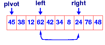
Most implementations of quick sort make use of the fact that you can partition in place by keeping two pointers: one moving in from the left and a second moving in from the right. They are moved towards the centre until the left pointer finds an element greater than the pivot and the right one finds an element less than the pivot. These two elements are then swapped. The pointers are then moved inward again until they "cross over". The pivot is then swapped into the slot to which the right pointer points and the partition is complete.

int partition( void *a, int low, int high )
  {
  int left, right;
  void *pivot_item;
  pivot_item = a[low];
  pivot = left = low;
  right = high;
  while ( left < right ) {
    /* Move left while item < pivot */
    while( a[left] <= pivot_item ) left++;
    /* Move right while item > pivot */
    while( a[right] > pivot_item ) right--;
    if ( left < right ) SWAP(a,left,right);
    }
  /* right is final position for the pivot */
  a[low] = a[right];
  a[right] = pivot_item;
  return right;
  }

Note that this above code does not check that left does not exceed the array bound. You need to add this check, before performing the swaps - both the one in the loop and the final one outside the loop. partition ensures that all items less than the pivot precede it and returns the position of the pivot. This meets our condition for dividing the problem: all the items in the lower half are known to be less than the pivot and all items in the upper half are known to be greater than it.
Note that we have used our ItemCmp function in the partition function. This assumes that there is an external declaration for ItemCmp and that in any one program, we only want to sort one type of object. Generally this will not be acceptable, so the formal specification for quicksort in the Unix and ANSI C libraries includes a function compar which is supplied to qsort when it is called. Passing the function, compar, which defines the ordering of objects when qsort is called avoids this problem in the same way that we passed an ItemCmp function to ConsCollection

Analysis

The partition routine examines every item in the array at most once, so it is clearly O(n). Usually, the partition routine will divide the problem into two roughly equal sized partitions. We know that we can divide n items in half log₂n times. This makes quicksort a O(nlogn) algorithm - equivalent to heapsort.
However, we have made an unjustified assumption - see if you can identify it before you continue.http://imraan-prrec.blogspot.in/2015/10/quick.html

Quick

7.3 Quick Sort (cont)

Quick Sort - The Facts!

Quick Sort is generally the best known sorting algorithm, but it has a serious limitation, which must be understood before using it in certain applications. What happens if we apply the qsort routine on the previous page to an already sorted array? This is certainly a case where we'd expect the performance to be quite good!
However, the first attempt to partition the problem into two problems will return an empty lower partition - the first element is the smallest. Thus the first partition call simply chops off one element and calls qsort for a partition with n-1 items! This happens a further n-2 times! Each partition call still requires O(n) operations - and we have generated O(n) such calls.

In the worst case, quicksort is an O(n²) algorithm!

Can we do anything about this?

A number of variations to the simple quicksort will generally produce better results: rather than choose the first item as the pivot, some other strategies work better.

Median-of-3 Pivot

For example, the median-of-3 pivot approach selects three candidate pivots and uses the median one. If the three pivots are chosen from the first, middle and last positions, then it is easy to see that for the already sorted array, this will produce an optimum result: each partition will be exactly half (±one element) of the problem and we will need exactly ceiling(logn) recursive calls.

Random pivot

Some qsort's will simply use a randomly chosen pivot. This also works fine for sorted arrays - on average the pivot will produce two equal sized partitions and there will be O(logn) of them.

However, whatever strategy we use for choosing the pivot,
it is possible to propose a pathological case
in which the problem is not divided equally at any partition stage. Thus quicksort must always be treated as potentially O(n²).

Why bother with quicksort then?

Heap sort is always O(nlog n): why not just use it?

Heap

Algorithms for Sorting - Heapsort

Heapsort

Based on Priority Queues
Sorts in O(NlogN) time by performing N times deleteMin operations.
Why O(NlogN)?

Each deleteMin operation takes logN running time.
N times performing deleteMin → NlogN running time

Basic algorithm (not very efficient - extra memory required):

Store N elements in a binary heap tree.
Perform deleteMin operation N times, storing each element deleted from
the heap into another array.
Copy back the array.

Improvements: Use the same array to store the deleted elements
instead of using another array
How can we do this?
After each deletion we percolate down the hole that is formed after the deletion,
and as a result we get a vacant position in the array - the last cell.
There we store the deleted element.
When all the elements are deleted and stored in the same array following the above method,
the elements will be there in reversed order.
What is the remedy for this?

Store the elements in the binary heap tree in reverse order of priority -
then at the end the elements in the array will be in correct order. Complexity of heap sort: O(NlogN) is the rough estimate.
Here is an example of heapsort.

Learning Goals

Be able to explain how heapsort works and its complexity.

Exam-like questions

Explain the complexity of heapsort
Given an array e.g. 17, 23, 10, 1, 7, 16, 9, 20, sort it on paper using heapsort
Write down explicitly each step.

Heap

An Example of Heapsort:
Given an array of 6 elements: 15, 19, 10, 7, 17, 16, sort it in ascending order using heap sort.
Steps:

Consider the values of the elements as priorities and build the heap tree.

Start deleteMin operations, storing each deleted element at the end of the heap array.

After performing step 2, the order of the elements will be opposite to the order in the heap tree.
Hence, if we want the elements to be sorted in ascending order, we need to build the heap tree
in descending order - the greatest element will have the highest priority.
Note that we use only one array , treating its parts differently:

when building the heap tree, part of the array will be considered as the heap,
and the rest part - the original array.

when sorting, part of the array will be the heap, and the rest part - the sorted array.

This will be indicated by colors: white for the original array, blue for the heap and red for the sorted array
Here is the array: 15, 19, 10, 7, 17, 6

Building the heap tree